RO system calculations: recovery, rejection, flux, pressure and energy

1. Recovery and concentration factor

Recovery R = Qp / Qf × 100%; concentration factor CF = Qf / Qc = 1 / (1 − R).

For 75 m³/h permeate from 100 m³/h feed: R = 75%, CF = 4, and the concentrate salinity is roughly 4× the feed (slightly less in practice because salt also leaves with the permeate; the exact value needs a solute balance).

System recovery is not the sum of stage recoveries — it is total permeate over total feed after all stages in series. Concentrate recirculation, two-pass systems and concentrate reuse all change the number, so draw the actual flow scheme before calculating.

2. Flux and membrane area

Average flux J = Qp / A_total, in LMH (L/m²·h) or GFD (gal/ft²·d). Conversion: 1 GFD ≈ 1.698 LMH.

Example: 100 m³/h permeate over 6000 m² of membrane gives J = 100000 / 6000 ≈ 16.7 LMH ≈ 9.8 GFD.

Element count N = A_total / A_element. A 400 ft² element is about 37.2 m², 440 ft² about 40.9 m², 365 ft² about 33.9 m². Round the result to whole pressure vessels (usually 6 elements per vessel).

3. Rejection and permeate TDS

Rejection = (1 − Cp / Cf) × 100%, where Cp is permeate TDS and Cf is feed TDS.

Three things to keep in mind:

• System rejection is not the element's nominal rejection. The nominal value is measured under standard test conditions (typically 2000 mg/L NaCl, 25 °C, 15% recovery, a specified pressure). Because concentrate is formed and stages are in series, system rejection is normally a little lower than the single-element figure.
• Permeate TDS must be flow-weighted. Each stage produces different permeate quality; only the blended total is a delivery figure.
• Warmer water lowers rejection. Salt passage rises about 3% per °C while water flux also rises, so permeate TDS degrades noticeably with temperature.

4. Osmotic pressure and net driving pressure

Empirical osmotic pressure: π ≈ 0.7 × TDS(mg/L) / 1000 (bar, natural water approximation); a pure NaCl solution is about 0.85 bar per 1000 mg/L at 25 °C. Accurate values require summing ion activities — in practice use the ion model in vendor software.

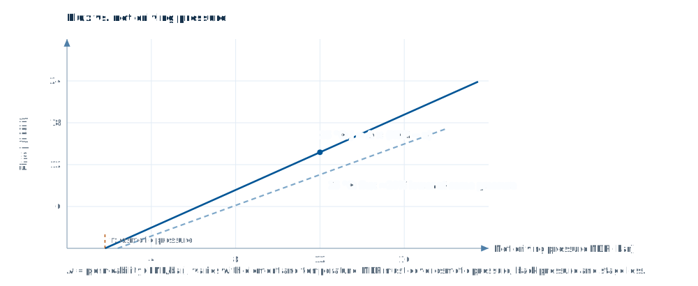
Net driving pressure: NDP = P_feed − ΔP_stage/2 − P_permeate − π_avg.

Here π_avg is the average osmotic pressure difference between the concentrate side of the membrane and the permeate side; in practice it is approximated as the arithmetic mean of feed and concentrate osmotic pressure minus permeate osmotic pressure. The higher the recovery, the larger π_avg, and the required feed pressure rises faster than intuition suggests — which is the main reason energy consumption climbs steeply at high recovery.

5. Pump power and specific energy

P(kW) = Qf(m³/h) × ΔP(bar) / (36 × η), with pump efficiency η typically 0.75–0.85.

Example: 100 m³/h feed, 15 bar pump head, η = 0.8 → P = 100 × 15 / (36 × 0.8) ≈ 52 kW. Specific energy = 52 / 75 ≈ 0.69 kWh/m³ of permeate.

Seawater systems run at 55–65 bar and typically use 3–4 kWh/m³, dropping to around 2.5–3 kWh/m³ with energy recovery. Brackish systems usually sit at 0.5–1.0 kWh/m³.

6. Temperature and ageing corrections

The temperature correction factor (TCF) comes from the manufacturer, normally referenced to 25 °C. As a rule of thumb flux falls about 3% per °C, so at 10 °C you get roughly 60% of the 25 °C flux. Design must check the local minimum monthly water temperature, not the annual average.

Ageing margin: after three years of operation flux typically drops 10–20% depending on cleaning and fouling, so the high-pressure pump should carry 10–15% head margin, or the design should be verified at end-of-life conditions.

7. A complete worked example

Conditions: feed TDS 1000 mg/L, 25 °C, 100 m³/h permeate, 75% recovery, 400 ft² brackish elements (37.2 m² each).

1. Feed flow Qf = 100 / 0.75 ≈ 133.3 m³/h; concentrate Qc ≈ 33.3 m³/h; CF = 4.
2. At a design flux of 17 LMH, A_total = 100000 / 17 ≈ 5882 m², N = 5882 / 37.2 ≈ 158 elements, rounded to 6 per vessel × 27 vessels = 162 elements (a 2:1 array would be 18 + 9 vessels).
3. Concentrate TDS ≈ 1000 × 4 × 0.97 ≈ 3880 mg/L (slightly below 4× once the solute balance is included).
4. Average osmotic pressure ≈ (1000 + 3880)/2 × 0.7/1000 ≈ 1.7 bar, with the permeate side ignored.
5. Allowing for stage pressure drop and back pressure, feed pressure lands around 8–10 bar (set by the element's flux–pressure behaviour).
6. Pump power ≈ 133.3 × 9 / (36 × 0.8) ≈ 42 kW, specific energy ≈ 0.42 kWh/m³.

This example only shows magnitudes and the order of operations. A real design solves flux, concentration and pressure drop for every element in every stage — which cannot be done by hand, and is the reason design software exists.